A conceptually simple(r) way to derive exponential shadow maps + sample code

A few months ago, while working on an improved version of exponential shadow maps, I stumbled on a new way to derive ESM equations which looks more simple and intuitive than previous attempts.

There is no need to invoke Markov’s inequality, higher order moments or convolutions. In fact all we have to do is to write the basic percentage closer filtering formula for equally weighted occluders and a receiver

The role of the step function is to perform a depth test on all occluders, depth test results are then averaged together to obtain a filtered occlusion term. The are many ways to write and a limit of exponential functions guarantees a fast convergence:

We can rewrite the original PCF equation as:

If we make the hypothesis that our shadow receiver is planar within the filtering window we are also implicitly assuming that the receiver is the most distant occluder (otherwise it might occlude itself, which can’t happen given our initial hypothesis), thus we have .
Armed with this new assumption we observe that the term quickly converges to zero for all occluders:

As we already know controls the sharpness of our step function approximation and can be used to fake soft shadows. Ultimately we can drop the limit and we obtain the ESM occlusion term formula:

Exponential shadow maps can be seen as a very good approximation of a PCF filter when all the occluders are located in front of our receiver (no receiver self shadowing within the filtering window). There’s not much else to add, if not that this new derivation clearly shows the limits of this technique and that any future improvements will necessarily be based on a relaxed version of the planar receiver hypothesis.

For unknown reasons some old and buggy ESM test code was distributed with ShaderX6. You can grab here the FxComposer 2.0 sample code that was meant to be originally released with the book.

Fast Percentage Closer Filtering on Deferred Cascaded Shadow Maps

Here’s a nice trick for whoever has implemented (as a single pass that operates in screen space) deferred cascaded/parallel split shadow maps on hardware that does not allow to index texture samplers associated with different view space splits.

One way to address this issue is to store multiple shadow maps (usually one per split) into a single depth texture, then the correct shadow map can be sampled computing (per pixel!) all the possible texturing coordinates per each split and selecting the right one through predication. Another method quite similar to the first one involves removing the predication step and replacing it with dynamic branches. This can end up being faster the the predication method on some hardware, especially if we have to select the correct sampling coordinates among many splits.

But what if we want to take a variable amount of PCF samples per split without using dynamic branching? (I love DB but it’s not exactly fast on every hardware out there, is up to you decide when it’s a good idea to use it or not).
It’s indeed possible to take a dynamic number of samples per pixel using an hardware feature that was initially introduced by NVIDIA to accelerate…stencil shadows! (ironic, isn’t it?)

I am talking about the depth bounds test which is a ‘new’ kind of depth test that does not involve the depth value of the incoming fragment but the depth value written in the depth buffer at the screen space coordinates determined by the incoming fragment. This depth value is checked against some min and max depth values; when it’s not contained within a depth region the incoming fragment gets discarded. Setting the depth min and max values around a shadow map split is a easy way to (early!) reject all those pixels that don’t fall within a certain depth interval. At this point we don’t need to compute multiple texture coordinates per pixel anymore, we can directly evaluate the sampling coordinates that map a pixel onto the shadow map associated with the current split and take a certain number of PCFed samples from it.

Multiple rendering passes are obviously needed (one per split) to generate an occlusion term for the whole image but this is not generally a big problem cause the depth bounds test can happen before our pixel shader is evaluated and multiple pixels can be early rejected per clock via hierarchical z-culling (this approach won’t be fast if our image contains a lot of alpha tested geometry as this kind of geometry doesn’t not generate occluders in the on chip hi-z representation forcing the hardware to evaluate the pixel shader and eventually to reject a shaded pixel).

The multipass approach can be a win cause we can now use a different shader per shadow map split making possible to take a variable number of samples per split: typically we want to take more samples for pixels that are closer to the camera and less samples for distant objects. Another indirect advantage of this technique is the improved texture cache usage as the GPU won’t jump from a shadow map to another shadow map anymore. In fact with the original method each pixel can map anywhere in our big shadow map, while going multipass will force the GPU to sample locations within the same shadow map/parallel split.

I like this trick cause even though it doesn’t work on every GPU out there it puts to some use hardware that was designed to accelerate a completely different shadowing technique. Hope you enjoyed this post and as usual comments, ideas and constructive critics are welcome!

Why GPUs are not (so) good at post processing images

Now I know the title of this post may sound controversial, but keep on reading, you might even end up agreeing with me.
Post processing effects are often implemented via convolutions, reductions and more sophisticated filters such as bilateral filters. What is interesting here is that the vast majority of these techniques all have something in common: data needed to work on a pixel are often required to work on neighboring pixels as well. This is an important property which is usually referred as ‘data locality’ and GPUs exploit it through texture caches.

Pixel shaders programming model has been designed to enable maximum parallelism. Each pixel is processed independently from any other pixel and no intercommunication is possible within a rendering pass. This model allows to pack an high number of processors on a single chip without having to worry about their mutual interactions, as no data synchronization between them is necessary..ever! This is also why the only atomic operations implicitly supported by current GPUs are related to alpha blending.

While this model has been incredibly successful it’s not exactly optimal when we would like to share data and computations across many pixels. As a practical example we can consider a simple NxN separable box filter which can be implemented on a GPU in two passes; each pass requires to fetch N samples and perform N-1 MADDs (or N-1 ADDs and one MUL) in order to compute a filtered pixel. This way to process data is clearly sub-optimal as while we move over the image horizontally or vertically each not-yet-filtered pixel shares N-1 neighboring pixels with the previously filtered pixel. Why wouldn’t we want to re-use those informations? Unfortunately we can’t, on a GPU..

..On the other hand modern multi-core CPUs can easily outperform GPUs in this case. Each core could be assigned to not overlapping areas of the image, moreover a pixel can accumulate its filtered value in a register and pass it to the next pixel.
At each iteration we wouldn’t need to fetch N samples anymore, we can in fact re-use the value generated by the previous iteration. As the filter kernel moves horizontally or vertically over the image at each new step an old pixel as to be removed from the accumulator and a new one can be added to it. Like in a fifo buffer we remove the first entry in the fifo and we add a new one (the fifo can be managed via registers rotations or using a modulo N-1 pointer to an array of values). At each step only one new value has to be read from memory (two if we implement it with a rotating pointer) and only one value has to be written to memory (or two again..). An addition, a subtraction and a multiplication would be needed per iteration to filter a pixel, no matter how wide our box filter is! More complex separable filters as tent or gaussian filters can be easily implemented multi-passing the work done on a column or a row of the image two or three times; for large filter kernels this is going to be incredibly fast as again the computation time does not depend by the filter width anymore

On a processor like CELL a single SPU would probably be able to perform such a task on single precision pixels at 4-5 cycles per pixel with fully pipelined and unrolled loops (data transfer from and to external memory are handled via asynchronous DMA operations). 6 SPUs could apply a box filter with ANY kernel size (even the whole screen!) on a 720p image over 40 times per frame, at 60 frames per second, and consuming only a relatively small amount of memory bandwidth as most read and write operations would happen on chip. This is admittedly a best case scenario, something slightly more complex would be necessary to also have a very good accuracy on the filtered data, but it’s clear that an architecture like CELL is very well versed in this kind of data processing. I hope to see more and more games in the future implementing their full post processing pipeline on CELL and off loading this way a ton of work from RSX that could then spend more time doing what it does best (e.g. shading pixels which don’t share a great amount of data and computations!)

It’s interesting to note that the last GPU architecture from NVIDIA (G8x) was also designed to be more efficient at tasks as image post processing. For the first time developers can leverage on a small on chip memory which is shared by a cluster of ALUs (each G8x GPU has a variable number of ALUs clusters..), each cluster has its own shared on chip memory which is split over multiple banks. As each memory bank can only serve one ALU per clock cycle it’s not certainly straightforward to make a group of processors use this memory without incurring in memory stalls or synchronization issues, nonetheless it looks we are at least going toward the right direction. Unfortunately at the time I’m writing this I’m not aware of any way to use these capabilities via some graphics API as D3D or OpenGL.

So.. do you still think GPUs rock at image post processing?;)
Feel free to post your own take on the subject, rants and errata corrige.

A (not so) little teaser

When it comes down to real time computer graphics, shadows rendering is one of the hottest topics. Shadow maps are currently the most used shadowing technique: they are reasonably fast, simple to implement (in their basic incarnations at least!) and unlike stencil shadows, they work even with not manifold meshes. Unfortunately shadow maps can look ugly as well, their resolution is never enough and all those aliasing and ‘acne’ problems drive people insane. This is why every year a lot of research goes into new shadowing techniques or into improving current ones. Papers and articles about shadow mapping often divide into two distinct groups:

1. How to improve virtual shadow maps resolution ( for example all the works about warped projection schemes belong to this category ).
2. How to improve shadow maps filtering quality/speed for hard edged and/or soft edged shadows

Personally, I find this second class of problems more interesting, cause it is still unknown territory and there is a lot of work to do about it.

A popular shadow maps filtering algorithm is percentage closer filtering, first developed by Pixar and later integrated by NVIDIA on their graphics hardware. It is based on taking a number of samples (the more, the better..) from a shadow map, performing a depth test with each of them against a shadow receiver and then averaging together all the depth test results.The key idea here is that filtering a shadow map, unlike what we do with colour textures, is not about directly filtering a bunch of depth values.Averaging together depth values and performing a single depth test on their mean value wouldn’t make any sense, cause a group of occluders which are not spatially correlated can’t be represented by a single averaged occluder. That’s why to have meaningful results filtering has to happen after depth tests, not before.

PCF is still the most used technique to filter shadow maps but a new algorithm called Variance Shadow Maps (developed by William Donnelly and Andrew Lauritzen) has deservedly attracted a lot of attention. VSM are based on a somewhat different and extremely interesting approach: depth values located around some point over a shadow map are seen as a discrete probability distribution. If we want to know if a receiver is occluded by this group of depth samples we don’t need to perform many depth tests anymore, we just want to know the probability of our receiver to be occluded or not. Constructing on the fly a representation of an unknown (a priori) discrete probability distribution it is basically an impossible task, so Donnelly and Lauritzen’s method doesn’t try to compute the exact probablity of being in shadow.

Chebyshev’s inequality is used instead to calculate an upper bound for this probability. This inequality categorizes a probability distribution using only two numbers: mean and variance, which can be easily computed per shadow map texel. Incidentally what we need to do in order to compute mean and variance is similar to what we do when we filter an image. So this new approach allows for the first time to filter shadow maps in light space as we do with colour images, and also enable us to use GPUs hardwired texture filtering capabilities to filter a variance shadow map.

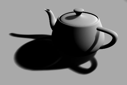
No wonder VSM triggered a lot of interest (a rapidly growing number of games is using this new techinque) as it has made possible what many, me included, thought was not possible. We can now apply filters to the variance shadow map and work with it as we were working with some colour texture. Here an example of the kind of high quality shadow that is possible to achieve filtering a variance shadow map with a 7×7 taps gaussian filter. In this case filtering has been applied with a separable filter so that we just need to work on 2N samples per shadow map texel instead of NxN samples that PCF would require.

Variance Shadow Maps – 7×7 Gaussian Filter

Memory requirements and hardware filtering issues aside VSM only significant flaw is light bleeding/leaking: a problem that manifests itself when shadows casted by occluders that are not relatively close to each other overlap over the same receiver.

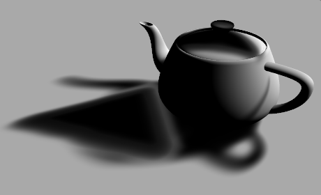
For example in this screen shot a triangle (not visibile in the image) located above the teapot is casting a shadow over the rest of the scene, and we can easily tell the shape of this new occluder by the lighter areas that are now inside the shadow casted by the teapot.

Variance Shadow Maps – Light bleeding caused by a second occluder

Occluders that overlap within a filtering region and that are not close to each other generate high depth variance values in the variance shadow map. High variance deteriorates the quality of the upper bound given by Chebyshev’s inequality, and since this inequality performs a conservative depth test, it can’t simply tell us if a point is in shadow or not. The amount of light leaking into shadows is directly proportional to the filter kernel size; this is what we get using a wider filter:

Variance Shadow Maps – More light bleeding with a 15×15 Gaussian Filter

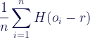
A well known work around for this issue is to over darken the occlusion term computed via Chebyshev’s inequality in order to reduce areas affected by light leaks. Over darkening can be achieved via 1D textures look-ups that encode a pre-defined and artist-controlled monotonic decreasing function or we can explicitly use functions such as or

This method doesn’t guarantee to eliminate light bleeding cause variance can’t really be bound in the general case (think about a mountain casting a shadow over a little town). Over darkening also destroy high frequency information in shadow silhouettes, at an extent that can transform high quality shadows in undefined dark blobs, which can be a nice side-effect in those applications where we are not trying to produce realistic shadows!

When I first found out about variance shadow maps I was so excited about this new way to address shadow maps filtering that I thought there must have been a way to improve this technique in order to reduce light leaks without resorting to over darkening. It is obvious that Chebyshev’s inequality is in some cases failing to produce a good upper bound for an occlusion term cause it has not enough information to work with. The first and the second raw moments are not sufficient to describe a probability distribution, in fact is fairly easy to construct whole families of distributions that generate the same first and second order moments! This is a clear case of bad lossy compression: we discarded too much information and now we realize more data are necessary to describe our depth distribution.

At the beginning the solution seemed so simple to me: two moments are not enough and higher order moments need to be accounted for.How many of them? I didn’t know.. but I also quickly realized that computing higher order moments and deriving any other quantity from them (skewness, kurtosis, etc..) is an extremely difficult task due to numerical issues.

There is also another problem to solve, and not a simple one by any mean. What are we going to do with the extra moments? how do we evaluate the probability of being in shadow? I couldn’t find in statistics and probability theory literature any inequality that could handle an arbitrary number of moments. Moreover even though inequalities that handle three or four moments exist, they are mathematical monsters and we don’t want to evaluate them on a per pixel basis. In the end I decided to give it a go only to find out that this incredibly slow and inaccurate extension to variance shadow maps was only marginally improving light bleeding problems, and in some cases the original technique was looking better anyway due to good numerical stability that was sadly lacking in my own implementation.

Having found myself in a cul de sac I tried something completely different such as defining ‘a priori’ the shape of the (not anymore) unknown depth distribution. The shape of this new object is controlled by a few parameters that can be determined fitting per pixel its raw moments to the moments of the real depth distribution. Unfortunately even in this case is extremely difficult to come up with a function that is flexible enojgh to fit any real world distribution and that at the same is not mathematically too complex (we like real time graphics, don’t we?). I ran experiments with a few different models; the most promising one was a 4 parameters model built upon a mixture of 2 gaussian distributions sharing the same variance but having different mean values. It worked very well when we only have two distinct occluders in the filtering window, but it looked awful everytime something a bit more complex came to play within the filtering window.

Ultimately I had to change direction a third time, going back to a variation of the first method that I previously (and stupidly) discarded without evaluating it. The approach is relatively simple, no monstrous equations involved, and in a very short time I got something up and running:

A new shadow map filtering method

As you can see this image is quite similar to the its counterpart rendered with variance shadow maps. It does not handle not planar receivers as good as VSM (note the shadow casted by the handle over the teapot) but in only requires two or four bytes per shadow map texel to work, as canonic shadow maps implementations. Mip mapping and filters in shadow map space work fine too, but the most relevant advantage of this new technique is that it’s completely light leaks free at overlapping shadows (and no over darkening is required, it just works!). The only observable light bleeding is uniformly diffused and only depends upon the relative distance between casters and receivers. It is completely controllable via a scalar value, so that we can trade sharper (but still anti-aliased) shadow edges for less light leaks.

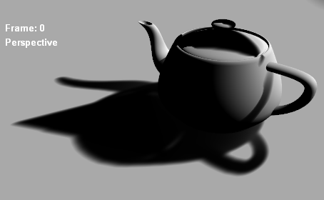
the malicious triangle is back but light leaks are no more!

Evaluating the occlusion term is also very cheap, it just requires a bunch of math ops and a single (at least bilinear filtered) sample from the shadow map, so that this technique is amenable to be implemented even on not very fast GPUs, as long as they support Shader Model 2.0. Although at this point in time I know why it doesn’t always do an amazing job I still have to find a way to fix the remaining problems without incurring in severe performance degradations. It is also easy to derive a ‘dual’ version of the orignal method that does not exhibit any of the previous issues but it also over darken shadows a bit too much.

I will post more about it in the future adding more information (still trying to improve it!) but all the details about it will be available next February when the sixth iteration of the Shader X books series will ship to bookstores.